Tracking gas mileage with Google Sheets

Copy our practice sheet and follow this post as we create a spreadsheet to track your car’s gas mileage. You will need to provide 4 simple variables every time you fill up. The formulas we create together will do the rest.

1. Date
2. Odometer Mileage
3. Gallons
4. Cost

If you make a habit of tracking these four variables it can help you better budget and track your car’s gas mileage. One of the many reasons we love Google Sheets is the accessibility of the software, you could enter all of this data from your phone as you fill up your car.

We have also added a bonus field to track the average gas price for your state, so you have an idea of what you should be paying or gas price trends.

Finding Cost Per Gallon

=IF(OR(ISBLANK(C2),ISBLANK(D2)),,D2/C2)

Formula Explained

The formula above will allow us to calculate the cost per gallon by dividing the total cost by the total number of gallons put in your vehicle. Note, column D holds the cost of filling up your car and column C holds the total amount of gallons of gas you filled your car with.

=D2/C2

=DIVIDE(D2,C2)

Both of the above formulas can be used to divide values in a cell.

This is the equation that provides the cost per gallon. This could be found using the DIVIDE function as well.

We want to avoid producing an error if we have yet to enter any data in a subsequent row. Otherwise, we would be dividing by a zero if we were to autofill our formulas down the column. Below are the errors for dividing by zero.

#DIV/0!

To avoid this error we use the additional functions.

• ISBLANK
• OR
• IF

=IF(OR(ISBLANK(C2),ISBLANK(D2)),value_if_true,value_if_false)

Formula Explained

To ensure we are only finding cost per gallon in rows with complete data we will use the ISBLANK function to return either a TRUE or FALSE statement. ISBLANK will return a TRUE statement if the referenced cell is empty or blank.

However, because we want to check if two cells are blank, we will utilize the OR function. The OR function returns a TRUE statement if any of the provided arguments are logically true.

=OR(ISBLANK(C2),ISBLANK(D2))

Now at this point we want to create a conditional statement using the IF function to either leave our Cost Per Gallon column blank or run our previous formula to return the cost per gallon. That is how we arrive at our final formula.

=IF(OR(ISBLANK(C2),ISBLANK(D2)),,D2/C2)

Miles Per Gallon (MPG)

The formula below can be used to track you cars MPG between each fill up. Where column B contains your car’s mileage and column C is your how many gallons you filled up your car with.

=IF(ISTEXT(B1),"N/A",IF(OR(ISBLANK(C2),ISBLANK(B2)),,ROUND(MINUS(B2,B1)/C2,2)))

Functions Used

• MINUS
• ROUND
• ISBLANK
• OR
• IF
• ISTEXT

Formula Explained

Our goal is to find our car’s miles per gallon (MPG), the number of miles a gallon of gas provides my car. Your car’s MPG can be effected by the driver, car maintenance, or terrain (city or highway driving), etc. This is why MPG can be variable or fluctuate between trips to the gas pump.

On the surface this is a simple equation. Take the miles between filling up and divide by the number of gallons needed to fill up.

=MINUS(B2,B1)/C2

The above formula will provide you with this solution. By subtracting your current odometer miles by the number of miles your odometer displayed at your last fill up, then dividing by the number of gallons it takes to fill up will provide you with your MPG.

However, you will notice that with just this equation we display many decimal places. There are a few ways to solve this issue. With a function or with Google Sheets build in tool.

Decrease Decimal Places

=ROUND(value,[places])

For formula clarity I chose to utilize the ROUND function and set the number of decimal places to 2.

=ROUND(MINUS(B4,B3)/C4,2)

Now, as we did in the previous step we will want to prevent this formula from displaying an error by setting a conditional statement.

=IF(OR(ISBLANK(C2),ISBLANK(B2)),,ROUND(MINUS(B2,B1)/C2,2))

Again, this formula will only return your vehicle’s MPG if the corresponding columns C and B contain data. This is a great way to autofill your formula down a column without producing errors and allowing your formulas to run as soon as the corresponding data is entered. This addition to our formula helps keep our spreadsheet clean and easy to digest.

The last issue we need to address is the fact that we can’t produce a MPG value for the first row of data. This is because our formula relies upon referencing the previous odometer value. Below are additional functions to address this concern.

=IF(ISTEXT(B1),value_if_true,value_if_false)

With this formula we are looking at the previous mileage value. If the previous mileage value contains text then we know that is the header to our spreadsheet and that there is no way to produce an MPG value.

ISTEXT is a function that will return a TRUE value if the referenced cell contains text. We then set an IF statement to run a formula dependent upon the value that is returned.

This addition also makes it simple to add simple text such as “Missed” to your spreadsheet to keep your data accurate and mileage between filling up correct.

=IF(ISTEXT(B1),"N/A",IF(OR(ISBLANK(C2),ISBLANK(B2)),,ROUND(MINUS(B2,B1)/C2,2)))

Now, we are able to combine our 3 formulas we developed into one formula. You will notice if the referenced Mileage cell is text then we will return the value “N/A” standing for “Not Applicable”. If column B’s referenced cell does not contain text then we will move on to our next formula, which includes another IF statement to evaluate if the corresponding mileage and gallon columns contain data. This is referred to as a nested function. By having two different IF statement conditions we are able to create more advanced formulas.

Finding Your Average MPG

We can now find your car’s average MPG. As stated before, your car’s MPG can vary between fill ups, so we will want to know an average to have a better idea of what to typically expect. Assuming column F contains your MPG values for each gas trip.

=IFERROR(AVERAGE(F2:F11),)

Functions Used

• AVERAGE
• IFERROR

With the AVERAGE function we can find the average value for all your car’s MPG values. We include an IFERROR function in our formula to return a blank value if our AVERAGE function returns an error. An error would occur if we have yet to enter any values in our spreadsheet.

Formatting Numbers in Google Sheets

Our average and miles per gallon columns are currently just digits. If you would like to add a unit to the end of these numbers, such as MPG, Google Sheets makes this an easy update.

1. Highlight the columns you would like to add a unit value to.
2. Select “Format” in the menu.
3. Hover over “Number”
4. Hover over “More Formats”
5. Select “Custom number format”

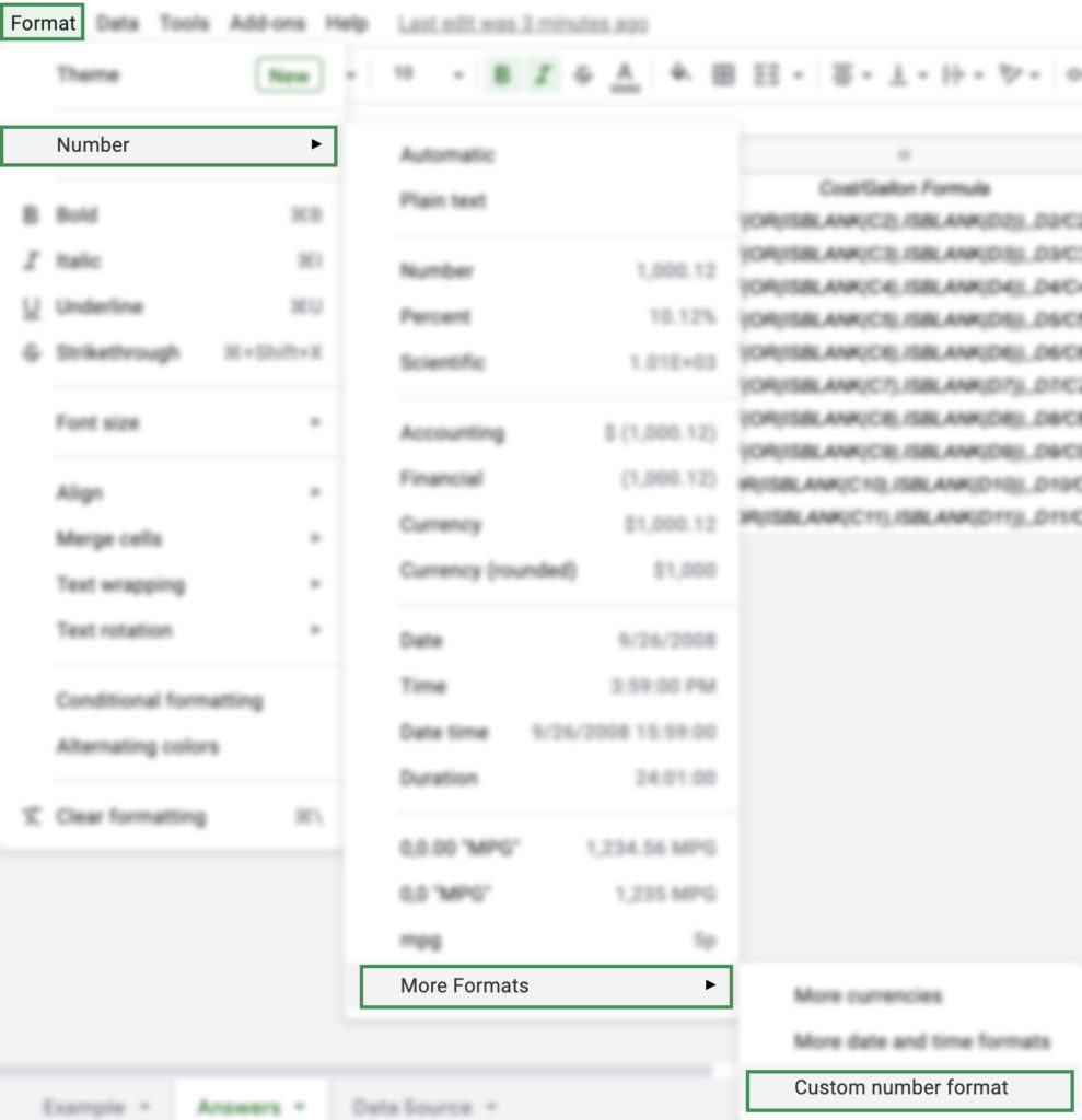
Enter this code to add “MPG” as a unit value to the end of your values.

0,0.00 "MPG"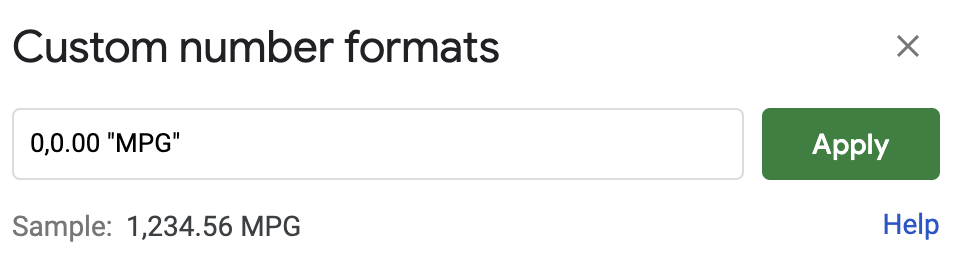

By using custom number formats to add our unit value, allows us to treat the columns as strictly numbers. Otherwise, we would be unable to find a columns average if we were to use a CONCATENATE function to add the unit value.

Practice Sheet

Bonus Formula

We have included two bonus formulas. One will import state average gas prices from this source and the other formula will find the average cost per gallon for your state and gas type. The data extracted from the source listed above will update automatically every day.

Importing Data with Google Sheets

Using the formula below we can import the current gas price for every state into a new tab.

=IMPORTHTML("https://gasprices.aaa.com/state-gas-price-averages/","table",1)

If you place this formula in a new tab it will extract the daily averages for gas prices for every state.

Formula Explained

With the IMPORTHTML function you can import a list or table from a URL. In the formula above we are requesting to pull data from the 1 instance of the table tag within our specified source URL. This extracts all the data from the table in the URL and places each data item in its own cell.

Expanding Our Formula

To make this data more accessible and digestible we are going to create a filter of sorts to only show relevant data to us. We will only want to see data from our state and of our gas type. To achieve this goal we will first create to variable drop downs using Data Validation.

Data Validation in Google Sheets

To create simple drop downs for our two variables, state and gas type we will use data validation.

1. Select the cell you would like your variable dropdown to populate.
2. Select “Data” from the menu.
3. Select “Data validation”
4. Leave criteria as “List from a range”
5. Select the range of cells that contain your desired variables.
6. Click “Done”.
7. Click “Save”.

Follow the same steps for both state and gas types. Now with these 2 variable cells easy to change with a dropdown menu, we can create a formula to utilize our new variable dropdowns.

=IFERROR(INDEX('Data Source'!A:E,MATCH(J2,'Data Source'!A:A,0),MATCH(K2,'Data Source'!A1:E1,0)),"Select From Dropdowns")	

Formula Explained

This formula works similarly to a VLOOKUP but is much more dynamic, typically referred to as an INDEX MATCH formula.

Functions Used

• INDEX
• MATCH
• IFERROR

Let’s start with the INDEX function. The INDEX function has three components.

1. Reference
2. Row (optional)
3. Column (optional)

In the formula above I’m indexing the entire table we imported at the start of the bonus function section. Next, I want to provide the row and column that coincide at the point of my state and gas type. By using the MATCH function we can return a cell location for matches.

So, for the second and third variable of our INDEX function we will be using match to find the row value of our state and the column value for our gas type.

=MATCH(J2,'Data Source'!A:A,0)

In the row portion of the INDEX function I’m using a MATCH function to find the state (J2) within the data set in my “Data Source” tab for column A and specified 0 because I want an exact match. This will return a single numerical value that will correspond to cell location for the state I specified in my dropdown menu we set up through data validation.

A similar use of the match function will be used to return the gas type.

=MATCH(K2,'Data Source'!A1:E1,0)

K2 is the variable I have select for my car’s gas type; regular, mid-grade, premium, diesel. The MATCH function will find the gas type across the top of our imported data set and return the column location with an exact match.

I added an IFERROR to encourage users to select their variables from the dropdown list and to prevent an error return when no variables are selected.

=IFERROR(INDEX('Data Source'!A:E,MATCH(J2,'Data Source'!A:A,0),MATCH(K2,'Data Source'!A1:E1,0)),"Select From Dropdowns")

INDEX MATCH formulas can seem complicated but they can make finding the cell position of your desired data you’d much easier to produce.

Please consider subscribing to our newsletter to receive expert tips and lessons like this one in your inbox.