Conditional formatting is a built in tool within Google Sheets that allows you to format a cell or range of cells based upon rules or conditions. If the conditions are met, then the cell will be formatted to your settings. Conditional formatting has many practical uses for beginner to advanced spreadsheets.
Conditional formatting is a great way to identify specific values or text, highlight trends or outliers in your data set, aesthetically improve your spreadsheets, and much more. Copy the practice sheet below to follow along as we review different conditional formatting examples and common uses.
Common Conditional Formatting Uses
- Format even rows
- Format specific text
- Format based on another column
- Format odd rows
- Format n smallest values
- Format duplicate values
- Format date range
- Format n largest values
- Format missing values
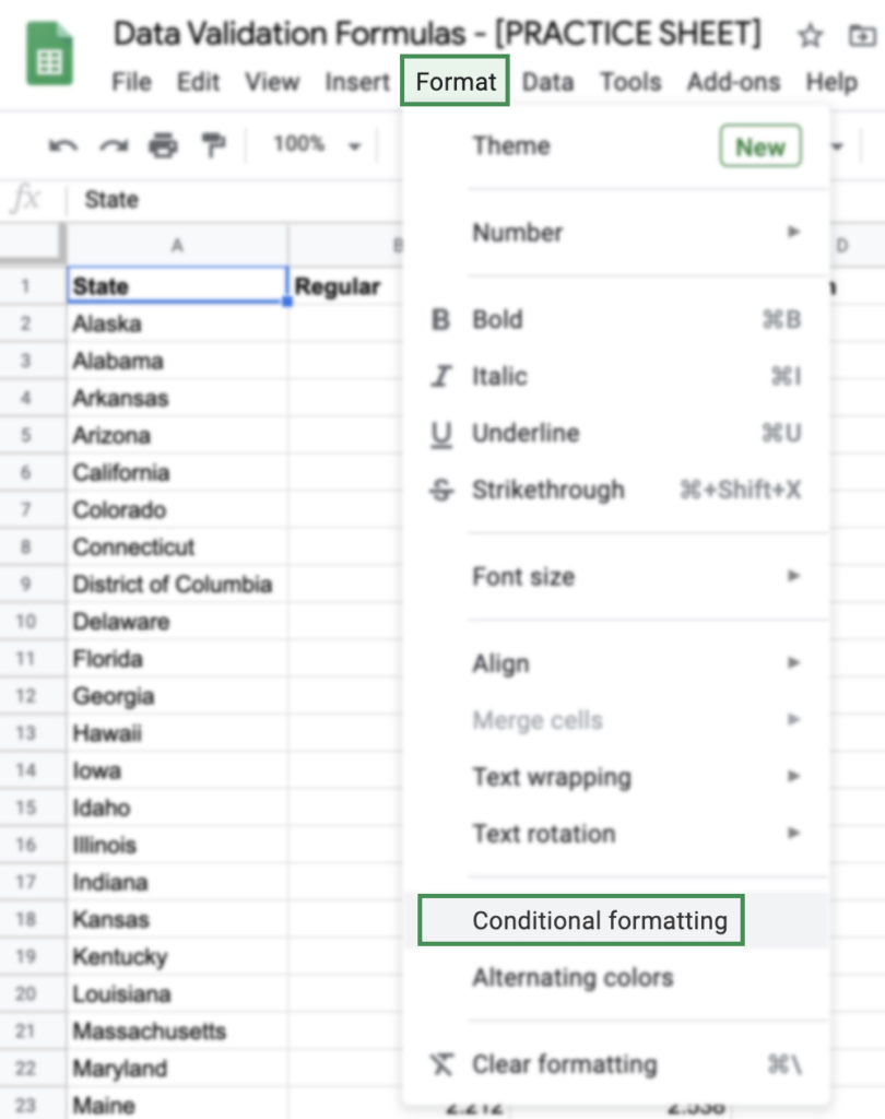
How To Access Conditional Formatting in Google Sheets
- Select the cell or cells you would like to apply your conditional formatting to.
- Select “Format” from the menu.
- Select “Conditional formatting”.
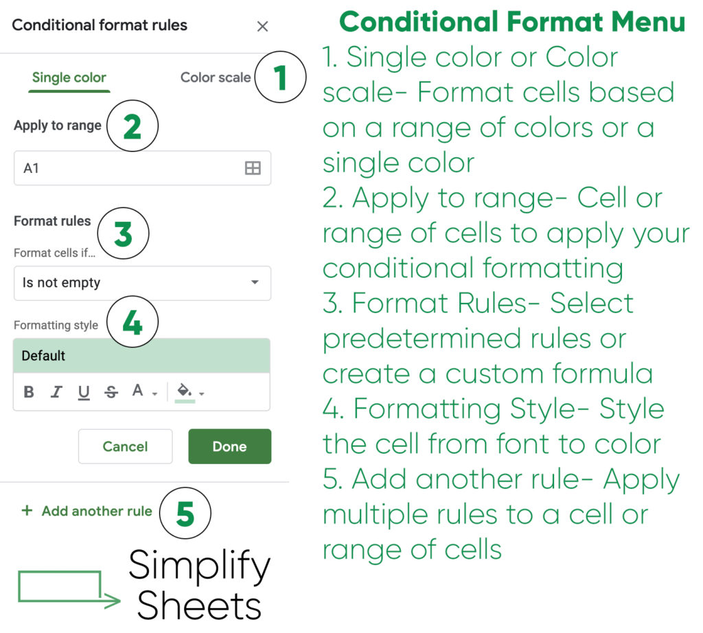
Areas of Conditional Formatting Menu
- Color rules- You can format a cell based on a single color or on a color scale.
- Apply to range- The cell or range of cells to apply your conditional formatting to.
- Format rules- There are 4 categories of the format rules; Text, Date, Number, and Custom Formula. These categories make it simple to create rules around common data values.
- Formatting style- Format the color and text of a cell.
- Add another rule- You can have multiple rules for a single cell or range. Keep in mind that color scale may be a solution if you need multiple rules to display different colors.
Conditional Formatting Rules
The conditional formatting rules are where you create the conditions that will format your cells. We previously mentioned there are 4 categories that these formatting rules fall into.
Let’s explore each of the rule categories to understand how they function and practical uses. Copy our practice sheet to follow along.
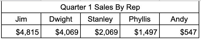
Practice Sheet Scenario
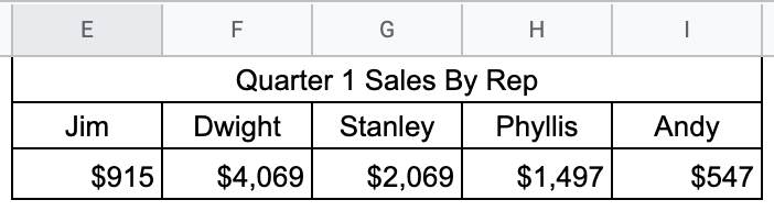
You are a paper sales man, Jim, and your boss is reviewing the quarter 1 sales. However, you notice that your Q1 sales are lower than expected. Conditional formatting can help you find these discrepancies.
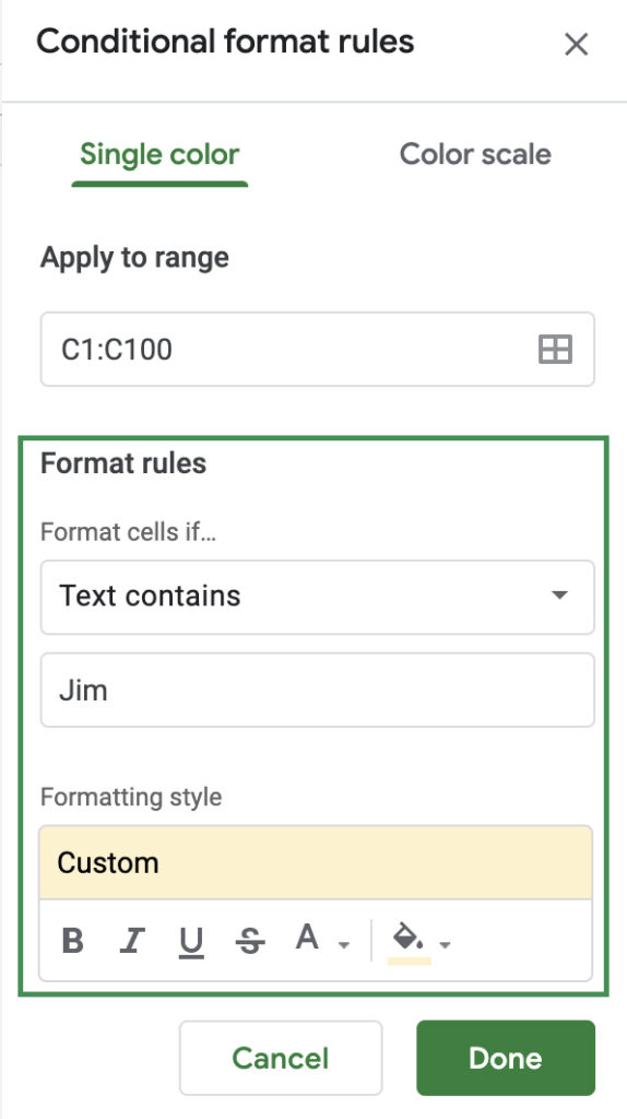
Text Based Rules
There are 7 predefined text based rules to create conditional formatting when a cell mets our criteria.
- Is empty
- Is not empty
- Text contains
- Text does not contain
- Text starts with
- Text ends with
- Text is exactly

These predetermined rules make identifying cells with consistent text patterns a breeze.
Practice Sheet Scenario
In the practice sheet you can see all of the logged sales for Q1. You are only concerned with your sales.
You start by highlighting all of the recorded sales for Q1 that are attributed to you using text based conditions.
Now you can see all of the sales that are attributed to you from the data set.
Date Based Rules
Date based rules are predetermined rules that expect cells containing date information. There are 3 main rules with 7 subset conditions.
3 main rules
- Date is
- Date is before
- Date is after
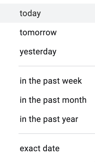
7 subset rules
- Today
- Tomorrow
- Yesterday
- In the past week
- In the past month
- In the past year
- Exact date
These predefined conditions make it simple to format cells that meet conditions based upon date values. These conditions also automatically update. For instance, if you want to always highlight data that is within the last week, your conditional format will automatically update each time you open your spreadsheet.
Practice Sheet Scenario
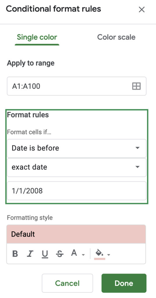
Now, we want to make sure all sales that have been entered are actually being recognized as 2008 quarter 1 sales. We will use a date conditional formatting rule to highlight any cells that were entered outside the date range of Q1.
To accomplish this we will create 2 conditional formatting rules for our date column. By utilizing Date is before and Date is after rules to quickly set conditions to highlight cells that were entered incorrectly and are actual Q 1 sales.
We see that two dates were entered incorrectly and were actually completed in Q1 but are outside of Q1’s date range. These sales were not being counted towards Jim’s total.
Number Based Rules
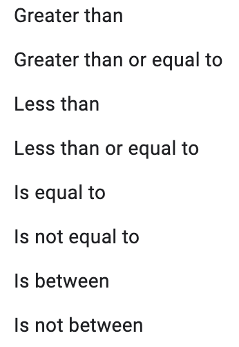
Number based rules allow you to format cells based on a numerical value. There are 8 predefined number based rules to conditionally format cells in Google Sheets.
- Greater than
- Greater than or equal to
- Less than
- Less than or equal to
- Is equal to
- Is not equal to
- Is between
- Is not between
This is a simple way to spot trends or unexpected values, especially for large data sets.
Practice Sheet Scenario
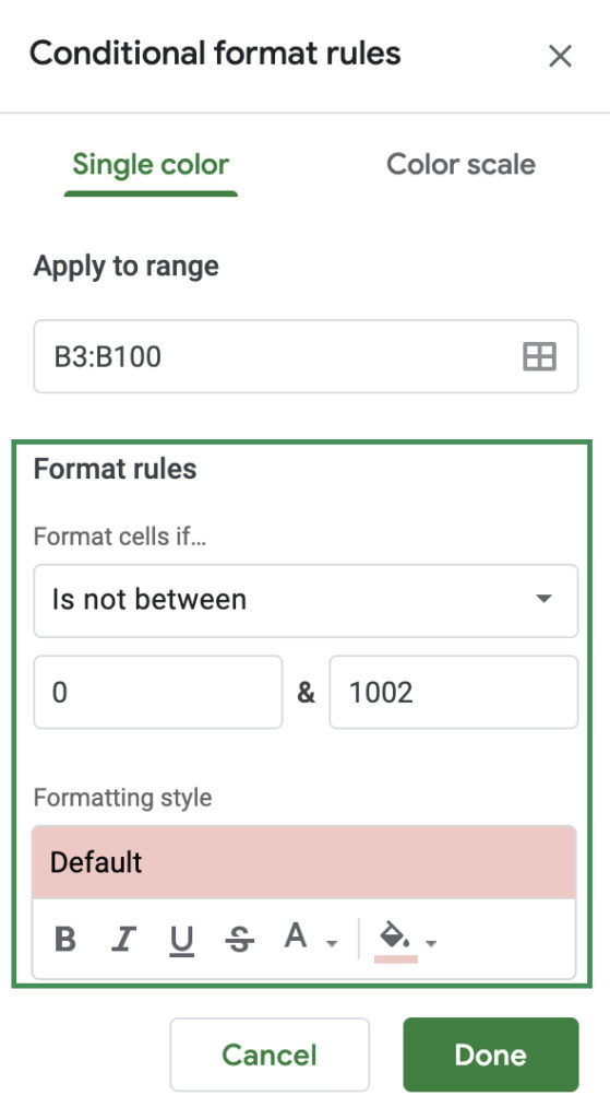
You remember the biggest deal you closed was with a phone book company for $1,002. Using a number based condition you can format any cells that fall outside the range of $0 and$1002.
You use the Is not between rule and set the values to 0 and 1002. Now cells outside this range are highlighted in red.
It’s easy to see now that some of your sales were entered as negatives or returns.
You share your new spreadsheet with the highlighted errors with your boss and the corrections are made. You now have the tools to find data that may be an outlier or have been entered incorrectly.
Conditional formatting within Google Sheets provides you with powerful tools to format cells based on rules.
Custom Formula
Custom formula allows you to format cells that satisfy the conditions of your formula. To format every other odd row you would use a formula as shown below. Google Sheets now offers a built in feature to alternate highlighting cells. See our additional uses at the top of this page to learn how custom formula conditional formatting can be used.
=MOD(ROW(),2)-1=0