How to find a person’s age with Google Sheets

Below is a simple formula to find a person’s current age using Google Sheets. Where A1 is the person’s Birthday.

=DATEDIF(A1,today(),"Y")

Formula Explained

Functions Used

• DATEDIF
• TODAY

With the above formula we are finding the difference between two dates; a birth date in cell A1 and today’s current date with the TODAY function. We are returning this difference in years ("Y").

Expanding Our Age Formula

The above formula is simple and effective, but by defining the goals of our formula we can expand our formula’s applications.

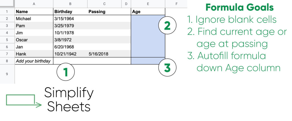
Formula Goals

Practice Sheet

Make a copy of our practice sheet to follow along as we expand our formula’s capabilities.

Ignoring Blank Cells

We want to create a formula that will not produce an age if the “birthday” cell is blank. This is a useful addition to our formula because it enables us to use the autofill feature for a whole column and not have to worry receiving errors or ages if there is no person in a row. This also allows us to add additional people to our spreadsheet and their age will be calculated once we enter a birthday. If we were to run the formula above with a blank “birthday” cell our formula would return a value of 120 or higher.

Functions Used

• IF
• ISBLANK

To ignore cells without a birth date we will use the IF and ISBLANK functions.

=IF(ISBLANK(A1),,DATEDIF(A1,today(),"Y"))

Formula Explained

The addition to our previous formula now features IF and ISBLANK functions. This formula will allow you to use the autofill function and only display an Age value for rows with a birthday. Assume A1 contains date of birth.

1. ISBLANK returns a boolean value of either TRUE or FALSE depending if the referenced cell is empty.
2. With the IF function we can now create two options for our formula.
   1. If ISBLANK(A1) is blank, then a value of TRUE is returned. This would result in the IF function returning the value_if_true value. This is the value after the first comma. Which we have specified to be blank. If there is no birthday we would like our age column to leave this cell blank.
   2. If ISBLANK(A1) is not blank, then a value of FALSE is returned. This would mean there is content within the birthday column, then the IF function returns the value_if_false value. In this case, this would run our previous formula to find the difference between the person’s birth date and today’s date and return the difference in years.

At this point you can use the autofill function for the entire “Age” column and it will only display ages for rows that have a birth date value.

Current Age or Age At Passing

Let’s consider you have a spreadsheet of family members’ birthdays and their contact information. You want to find everyone’s age or the age of family members when they passed away.

Functions Used

• IF
• ISBLANK
• DATEDIF

To expand our function to display the current age or age of passing, we need to create a formula to evaluate cells in the row to determine which formula to run.

=IF(ISBLANK(B1),DATEDIF(A1,TODAY(),"Y"),DATEDIF(A1,B1,"Y"))

Formula Explained

With this formula your Age column will return the person’s current age or if they have passed it will return the age of their passing. Assume A1 contains date of birth and B1 contains date of death.

1. ISBLANK returns a boolean value of either TRUE or FALSE depending if the referenced cell is empty.
2. With the IF function we can now create two options for our formula.
   1. If ISBLANK(B1) is blank, then a value of TRUE is returned. This would result in the IF function returning the value_if_true value. This is the value after the first comma. Which we have specified to return the person’s current age. If there is no date of death then we would like our age column to return the person’s current age.
   2. If ISBLANK(B1) is not blank, then a value of FALSE is returned. This would mean there is content within the date of death column, then the IF function returns the value_if_false value. In this case, this would run our new DATEDIF formula to find the difference between the person’s birth date and date of death and return the difference in years.

Combining Formulas

We created two formulas to address; blank cells, current age or age at death, and allowing for the formula to be copied down an entire column by returning a blank value when no data is in the Birthday column. We can now combine these two formulas into one and have a simple yet elegant formula that will give us a person’s age within Google Sheets.

=IF(ISBLANK(A1),,IF(ISBLANK(B1),DATEDIF(A1,TODAY(),"Y"),DATEDIF(A1,B1,"Y")))

Now our previous two formulas have been combined into one formula. You will notice, if done correctly, you have now created a nested IF statement. Nesting functions within one another is a tool that will help you advance your Google sheets skill set and enable you to create more advanced formulas.

Practice Sheet