Data validation is a powerful tool built into Google Sheets that allows for the easy creation of dropdown menus, checkboxes, data input checks, and more. Data validation is a great way to keep your spreadsheets organized and your data clean. Copy the practice sheet below to see the power of data validation and additional examples.
All data validations have been highlighted green. So, be sure to click on the green cells and then navigate to the data validation section to see how each validation is configured.
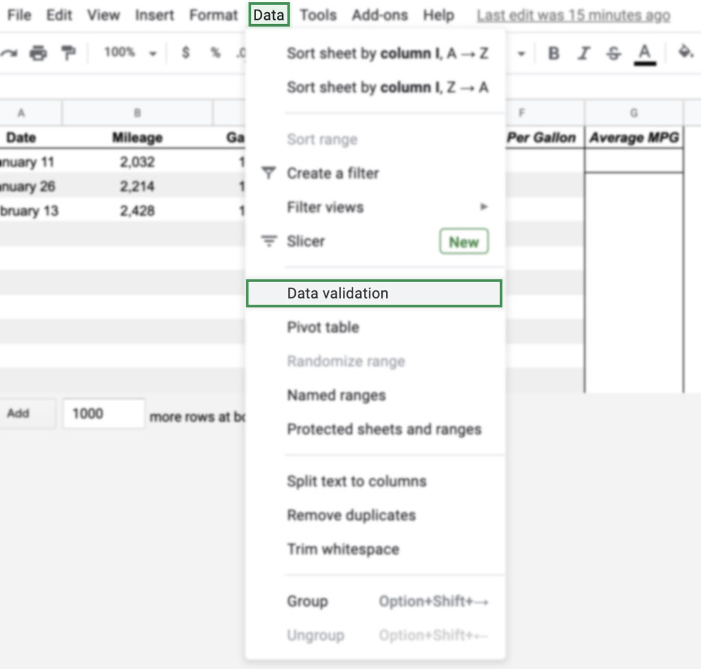
How To Access Data Validation
- Select the cell you would like to apply a data validation filter to.
- Select “Data” from the menu.
- Select “Data validation”.
The Different Areas of Data Validation
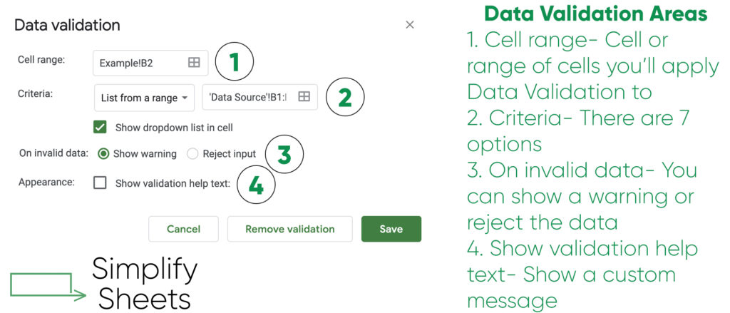
There are four main areas to the data validation menu. The “Show dropdown list in cell” is part of the Criteria area and that option will be different depending upon the selected criteria.
There are seven different types of data validation criteria. You can jump to a specific section to learn more.
Different Criteria of Data Validation in Google Sheets
List From A Range
This is far and away the most common data validation criteria we use at Simplify Sheets because it allows you to quickly add an extensive dropdown menu. But also, by setting a data validation for an entire column as your range you can easily include additional variables without having to reimplement your data validations. Imagine you track all sales leads in a spreadsheet and you assign a sales rep to each lead. With a data validation list from a range you can quickly add new sales reps and remove old reps to identify leads that need to be reassigned. Every additional item added to a data validation column will automatically be added to the dropdown list.
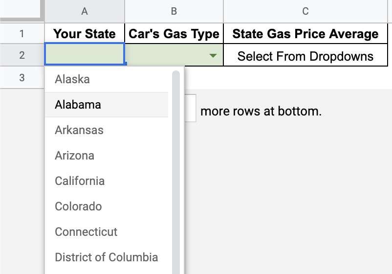
In the practice sheet you can see we created a dropdown using list from a range as the criteria. We are able to include all 50 states in a simple dropdown in a few clicks.
Our data validation dropdown list was created from a range of variables in a separate tab. A great way to keep your spreadsheet organized.
List Of Items
Setting your data validation criteria to list of items can be very quick and effective data validation technique. You write out a list of items that are acceptable within a cell or range, this too can have a drop down functionality. This is common for simple dropdowns; Yes or No, Mr. or Mrs., On-Time or Tardy, etc. This is a quick solution if you don’t want to place the variables in additional cells or a new tab.
In our example we need to quickly assign individuals to a soccer team.
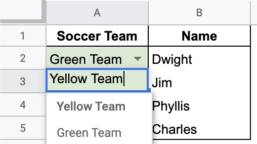
However, we recommend generating your dropdowns using the list from a range criteria. This is because it is easier to expand your acceptable variables. We typically keep a variable tab in our spreadsheet to quickly add to our data validations.
Take for example, if we were to expand our previously listed items; Yes or No or In-Progress, Mr. or Mrs. or Miss, On-Time or Tardy or Absent, etc. To expand these validations we need to reselect all of the cells, enter the data validation menu, and type or copy the additional variables. But you can see this can become rather tedious as your list continues to grow. A range makes it simple to see what data validation variables are already accepted and gives you the ability to quickly add more variables to your dropdown lists.
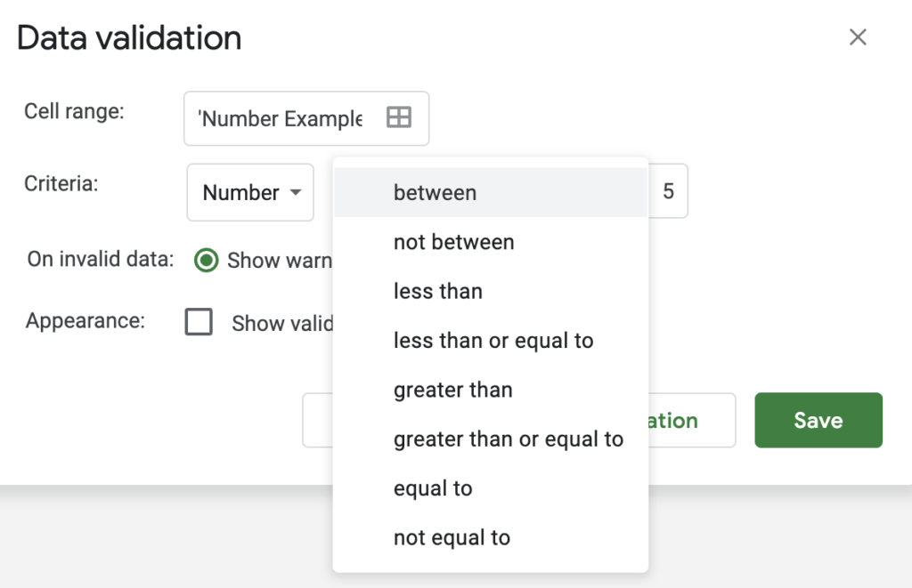
Number
Number criteria allows you to place a data validation, acceptable numerical values for a cell or range, to only accept a numerical value that satisfies your data validation’s rule. You can add additional rules to the acceptable digits. The predetermined criteria are:
- Between
- Not between
- Less than
- Less than or equal to
- Greater than
- Greater than or equal to
- equal to
- not equal to
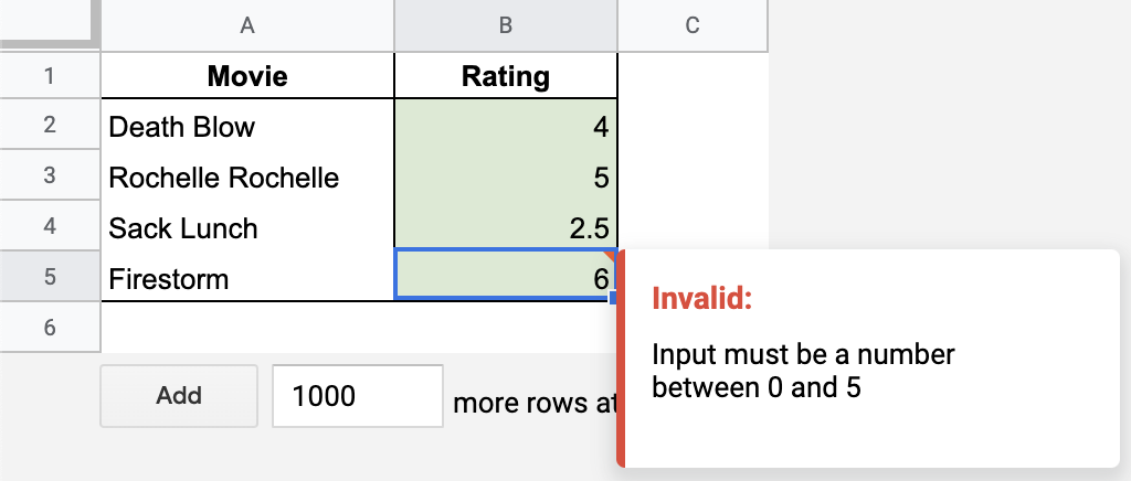
This can be useful to help keep your data clean. For instance, if you are grading tests and recording scores in a Google Sheets spreadsheet. With a number data validation you could be alerted if a value was entered outside the range of 0 to 100. This can save you and your graders time from having to rectify a discrepancy.
In our example we only want to provide movie ratings between 0 and 5. You can see a simple error message that alerts the user to data that is outside our acceptable limits.
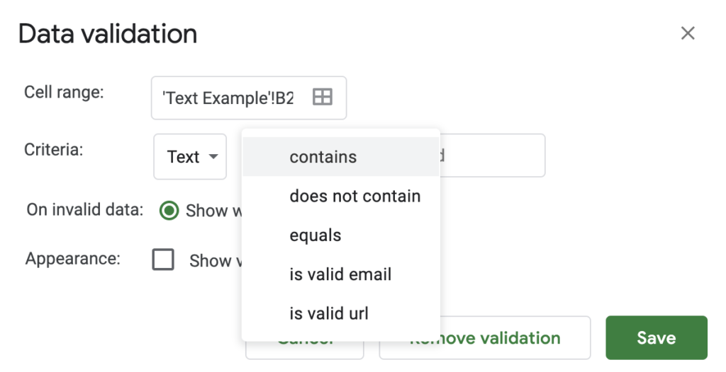
Text
Text works in a similar way as the number criteria but for text based rules. Like the number criteria there are additional predetermined criteria variables.
- Contains
- Does not contain
- Equals
- Is valid email
- Is valid URL
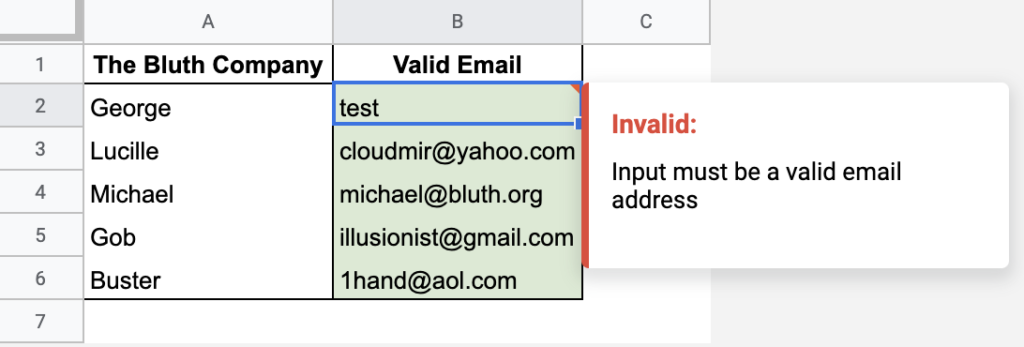
Again, another great way to use data validation in Google Sheets to ensure your entered data is an expected value. The valid email and URL check are especially useful when managing sales lists (client emails or prospective client websites) or collecting contact information at an event. This data validation will prevent a user from accidentally forgetting their email provider (gmail, yahoo, aol, etc.).
In our practice sheet you can see an example of the error message that would be populated if a user entered an invalid email address for cells with the data validation criteria set to “is valid email”. Keep in mind this will not check if the email exists, rather if it includes the expected characters of an email address.
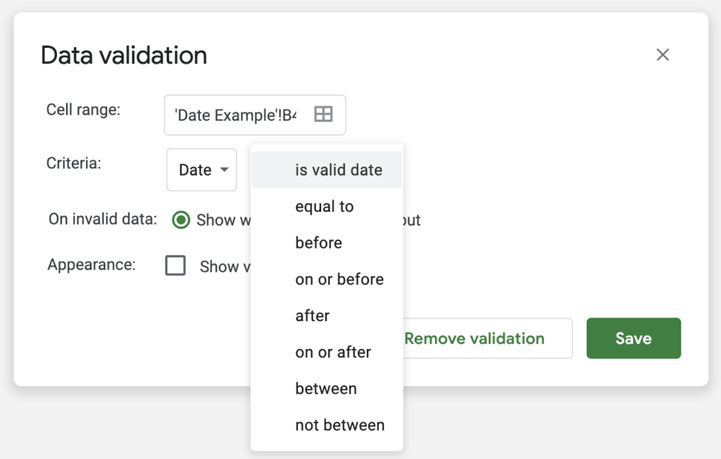
Date
Date criteria works as you’d expect, by ensuring the entered data within a cell or range of cells contains an acceptable date value. Again, there are some predefined criteria fields to set rules for acceptable data. This will help organize your data and ensure only expected values are entered into your spreadsheets.
- Is valid date
- Equal to
- Before
- On or before
- After
- On or after
- Between
- Not between
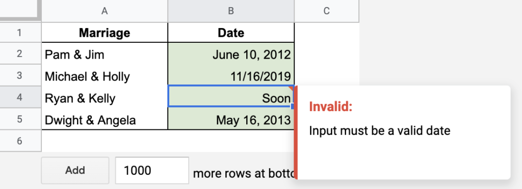
The date data validation can be a handy failsafe if you have additional formulas referencing your date information. A formula using a SUMIF function could incorrectly count total sales for a date range, if the referenced date cell isn’t a valid date. This could easily happen if a user were to misspell a month or if a user were to enter a date on a leap year. Both of these instances, as seen below, would be caught by a date data validation criteria set to “is valid date”.
Febuary 14, 20202/29/2019To the right you can see how the error message would appear. Note, that dates can appear in different formats, but all of the approved dates would be treated the same if a formula were to reference the date cells.
Custom Formula Is
Custom formula is criteria for data validation allows you to enter your own formula. Below is our example custom formula.
=$B$1="No"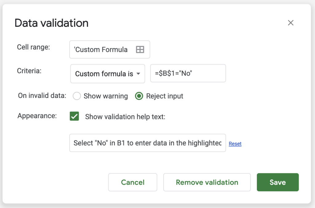
Notice, we are stating that if cell B1 equals “No” then we will accept data for the range of our data validation. We have an absolute reference to cell B1 by placing a $ in front of both the column and row cell reference.
If B1 were to equal anything other than the text “No” then our data validation would reject the input and show a custom validation help text.
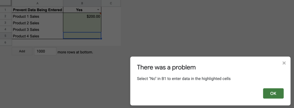
In our practice sheet we are preventing data from being entered until we change B1 from “Yes” to “No”. If B1 is set to “Yes” and you enter data in the highlighted green cells you will see the custom error message we wrote.
Checkbox
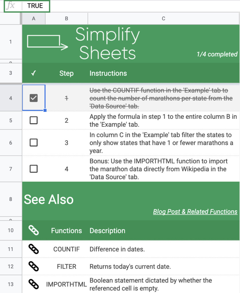
Checkbox is a useful data validation criteria that creates a simple checkbox that will check and uncheck with a simple click. At Simplify Sheets we use the checkbox data validation in all of our practice sheets. When we list our instructions we include a checkbox, so users can track their progress.
Note that when the checkbox is checked or unchecked the data validation treats this as either a “TRUE” or “FALSE” state. This enables you to reference your checkboxes as being complete or create conditional formatting depending upon the checkbox’s status. Both of these concepts are utilized in the image to the right.
Notice, that we have grayed out the checked boxes and placed a strikethrough the text of a completed task, this is accomplished with conditional formatting. At the top right corner there is a count of completed tasks, this is accomplished with a formula to count the number of completed tasks or TRUE values in column A.
All of this is only possible because the checkbox data validation returns a “TRUE” or “FALSE” value.
Now that you have an understanding of data validation and its different applications be sure to read up on conditional formatting and how they can be used together.