Below is a simple formula to separate a name into a First Name column and a Last Name column in Google Sheets. Where A1 is the cell containing the name you wish to separate.
=SPLIT(A1," ")Note the subsequent columns will need to be empty or you will see the following error. By simply removing the data in C1 and your SPLIT function will work as expected.
#REF!Error
Array result was not expanded because it would overwrite data in C1.

Formula Explained
Function Used
SPLIT
The SPLIT function will split the contents of the referenced cell by the specified delimiter. In the formula above we are splitting the contents of A1 by every space present in A1. This works great for cells containing first and last names or even first, middle, and last names. SPLIT is a great solution as long as all the content in column A is consistent. However, if the column you are attempting to separate has varying data another formula will need to be used.
Expanding Our Name Splitting Formula
Let’s say you have a column of names, but some cells have a middle name or initial while others just have a first name and some cells have a first and last name. Let’s create some additional formulas to address this situation.
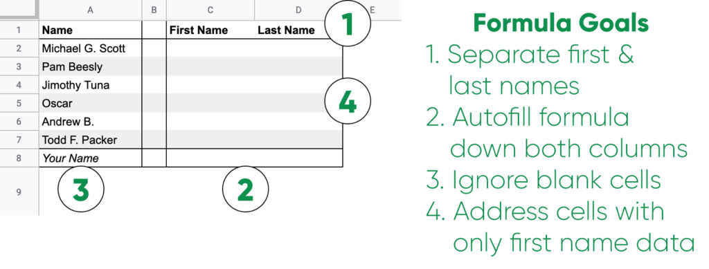
Formula Goals
- Separate first names into a new column
- Separate last names into a new column
- Utilize the autofill feature
- Ignore blank cells
- Function properly if only a first name is entered
Practice Sheet
Make a copy of our practice sheet to follow along as we work on adding additional formulas. In our practice sheet we are assuming that the first word in the cell corresponds to a person’s first name and the last word in the cell corresponds to the person’s last name.
Separate First Name
Let’s start with separating the first name or word in a cell into another column. We will accomplish this by referencing all characters after the first space in cell A1, which contains a person’s full name.
=IFERROR(IF(ISBLANK(A1),, LEFT(A1,FIND(" ",A1)-1)),A1)Functions Used
Formula Explained
Our formula’s first goal is to find the first space in cell A1. To accomplish this we will use the FIND function to return the position in cell A1 of the first space. The FIND function will return a numerical value.
We can then subtract 1 from the value our FIND function produced, to specify the number of characters we would like our LEFT function to extract. Below is our formula to pull the first name or word from cell A1.
=LEFT(A1,FIND(" ",A1)-1)Let’s expand our formula to account for cells that only have a first name or that are blank to prevent our formula from displaying an error.
Ignoring Blank Cells
We can expand our previous formula to ignore cells in column A that are blank with a few functions.
Additional Functions
The addition to our previous formula now features IF and ISBLANK functions. This formula will allow you to use the autofill function to only display a first name value for rows with text in column A.
=IF(ISBLANK(A2),, LEFT(A2,FIND(" ",A2)-1))ISBLANKreturns a boolean value of either TRUE or FALSE depending if the referenced cell is empty.- With the
IFfunction we can now create two options for our formula.- If
ISBLANK(A1)is blank, then a value of TRUE is returned. This would result in theIFfunction returning thevalue_if_truevalue. This is the value after the first comma. Which we have specified to be blank. If there is no name in column A we would like our first name column to leave the formula cell blank. - If
ISBLANK(A1)is not blank, then a value of FALSE is returned. This would mean there is content within the name column, then theIFfunction returns thevalue_if_falsevalue. In this case, this would run our previous formula to find the numerical position of the first space, subtract 1, and return all characters to the left of the first space.
- If
Only First Name Data
If certain cells only contain a first name and no additional data our current formula will result in an error. This is because our FIND function was unable to locate a space. However, because of our previous step we know their is data in the referenced cell or it would have remained empty and not produced an error.
So we are able to assume the referenced cell just contains a first name.
Additional Function
IFERROR
We know if an error is produced by our current formula then the cell just contains the person’s first name. By using the IFERROR function to provide content for the cell if an error is produced. The formula will return the data from A1 if our formula produces an error.
=IFERROR(IF(ISBLANK(A1),, LEFT(A1,FIND(" ",A1)-1)),A1)Separate Last Name
Separating the last name or word from a cell presents its own unique challenges. To accomplish pulling only the final word or name from a cell we are going to insert additional spaces between each word, then extract data starting from the right characters within the referenced cell, and finally trim the content to a single word.
=IF(ISERROR(SEARCH(" ",A1)),,TRIM(RIGHT(SUBSTITUTE(A1," ",REPT(" ",LEN(A1))),LEN(A1))))Formulas Used
LENREPTSUBSTITUTERIGHTTRIMSEARCHISERRORIF
Formula Explained
By establishing the goals of our last name formula we can construct a formula to accomplish our goals. The first goal of our formula is to separate each word enough to allow us to extract characters starting from the right side of our referenced cell. This formula will produce the last word or name of cell A1.
=TRIM(RIGHT(SUBSTITUTE(A1," ",REPT(" ",LEN(A1))),LEN(A1))- The first step in this formula is to use the
LENfunction to find the number of characters in cellA1.LENwill return a numerical value of all characters including spaces in the referenced cell. Example: “Simplify Sheets” would return aLENnumerical value of 15. - Next we will use the
REPTfunction to repeat a specified value, in this case a space, by the numerical value we found in step 1. - Use the S
UBSTITUTEfunction to replace all instances of spaces in the referenced cells. This will now separate each word in the referenced cell by the same number of spaces as the numerical count of characters in the referenced cell. Example: “Simplify Sheets” would now have 15 spaces between the two words. - With the
RIGHTfunction we are able to extract data starting from the right side of a cell by the number of specified character count. By setting the character count toLENof the referenced cell ensures we are only extracting the last word or name from the referenced cell. Example: Since we now have 15 spaces between “Simplify Sheets” and we extract 15 characters from the right we extract “Sheets” with 9 spaces in front of our last word. The word “Sheets” is 6 characters, which is why we have an extra 9 spaces at the beginning of our extracted value. - To remove the extra spaces from the beginning of our extracted value we use the
TRIMfunction.TRIMremoves leading, trailing, and repeated spaces in text.
Let’s expand our formula to address a few potential issues. In our first name formula we accept that if there is only one name in the referenced cell than it is the first name. In that case we will want to leave the last name cell blank.
Additional Functions
SEARCHISERRORIF
There are 2 potential issues we hope to address by expanding our function.
- If the referenced cell only contains a first name.
- If the name cell is blank.
=IF(ISERROR(SEARCH(" ",A1)),if_ture_value,if_false_value)Formula Explained
- By using the
SEARCHfunction we are able to search for a specific character within a referenced cell. By searching for a space if the referenced cell doesn’t contain a space it is either blank or a first name and will return an error. - With the
ISERRORfunction we are able to produce a boolean statement; if an error value is returned than this function produces a TRUE statement. If an error is not returned then it produces a FALSE statement. - With an
IFfunction we can specify values or formulas to run.
Combining our formulas
We can now combine our previous two formulas to produce a single formula that will return the last name or word in a cell, ignore blank cells, and return an empty value if the referenced cell only contains a first name.
=IF(ISERROR(SEARCH(" ",A1)),,TRIM(RIGHT(SUBSTITUTE(A1," ",REPT(" ",LEN(A1))),LEN(A1))))